Chapter 2: Foundations
This chapter introduces the concepts that the remainder of the thesis builds on, for readers without a background in machine learning. Sections 2.1 to 2.3 explain how large language models (LLMs) work and introduce prompting, the means by which the main experiments adapt a model to its task. Section 2.4 defines LLM agents and the planning horizon, the dimension studied by the third research question. Sections 2.5 and 2.6 contrast the optimisation of model weights with the optimisation of prompts and present the prompt optimiser GEPA as published. Section 2.7 introduces state-space search and exact solvers, which provide the ground truth against which the agents are measured on single floors.
2.1 From Language Models to Large Language Models
A language model assigns a probability to a sequence of text. Most modern language models do so one piece at a time: given the text so far, they predict a probability distribution over what comes next. For a sequence of units , the probability of the whole sequence is factorised into a product of such next-unit predictions:
The units are called tokens. A tokenizer splits text into tokens from a fixed vocabulary of subword pieces, so that frequent words are single tokens and rare words are split into several pieces (Sennrich et al., 2016). Numbers, coordinates and game terms such as "Slime Lord" therefore occupy one or more tokens, and every length limit discussed in this thesis is measured in tokens, not words.
A language model is implemented as a neural network: a function with a large number of adjustable numbers, called parameters, whose values are learned from data. The parameter count is the usual measure of model size; the largest model used in this thesis has 397 billion parameters. Before the network can process a token, the token is mapped to a vector of numbers, its embedding, which the network learns so that tokens used in similar contexts receive similar vectors.
Earlier language models counted how often short word sequences occur (n-gram models). Later models processed the text one token after another with a recurrent network that carried a summary of everything read so far (Jurafsky and Martin, 2025). Both approaches struggle with long-range dependencies, because information from early in the text must survive many processing steps to influence a later prediction.
2.1.1 The Transformer
The transformer (Vaswani et al., 2017) replaced step-by-step processing with self-attention: every token can draw information directly from every other token in the input. For each token, the network computes three vectors from its embedding: a query (what the token is looking for), a key (what the token offers) and a value (the information it passes on). Stacking these vectors for all tokens into matrices , and , attention is computed as
where is the length of the key vectors. The product scores how relevant every token is to every other token. The softmax turns each row of scores into weights that sum to one, and the result is a weighted mixture of the value vectors. Each token's new representation therefore depends on the whole input, weighted by relevance. A transformer runs several such attention functions in parallel (multi-head attention), follows them with a small feed-forward network, and stacks dozens of these layers (Figure 2.1).
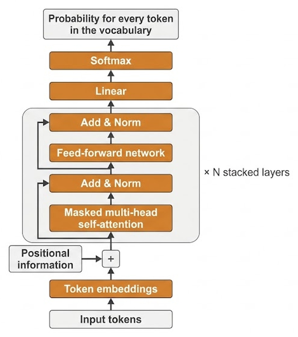
Figure 2.1: Simplified decoder-only transformer, after Vaswani et al. (2017). The input tokens are mapped to embeddings, to which information about each token's position in the text is added. Each of the stacked layers applies masked multi-head self-attention, through which every token attends to all earlier tokens, and then a feed-forward network. After each of the two, "Add & Norm" adds the input of the step to its output and normalises the result. The final linear layer and softmax produce a probability for every token in the vocabulary.
The original transformer had two parts: an encoder that reads an input sentence and a decoder that writes an output sentence, as needed for machine translation. Most current LLMs, including every model of the main experiments, keep only the decoder. A decoder-only model reads the text so far and predicts the next token; its attention is masked so that a token can only attend to tokens before it. Text is generated by appending the predicted token and repeating.
2.1.2 From Transformers to LLMs
Three developments turned the transformer into the LLMs in use today. First, pre-training on very large text corpora: the model learns to predict the next token on a large part of the public web, books and code, without any task-specific labels. Brown et al. (2020) showed with GPT-3, a 175-billion-parameter decoder-only model, that such a model can perform new tasks from a textual description and a few examples, without any change to its parameters. Second, instruction tuning: continued training on many tasks phrased as instructions makes the model follow instructions it has not seen before (Wei et al., 2022a). Training from human preference judgements makes its answers more helpful (Ouyang et al., 2022). Instruction-tuned models are used as chat models: the input is a sequence of messages from a system (standing instructions), a user (the current request) and the assistant (the model's earlier replies). Third, scale: parameter counts grew from millions to hundreds of billions.
Two further properties matter for this thesis. The context window is the maximum number of tokens the model can attend to at once. Everything the model knows about the current game must fit into it, including the instructions, the game state and any earlier turns. Models also use information in the middle of a long context less reliably than information at its start or end (Liu, N. F. et al., 2024). A mixture-of-experts (MoE) model replaces the single feed-forward network of a layer by many smaller "expert" networks and a router that sends each token to only a few of them (Shazeer et al., 2017). Only a fraction of the parameters is active for each token, which makes a very large model affordable to run. Model names reflect this: Qwen3.5-397B-A17B has 397 billion parameters in total, of which about 17 billion are active per token. A model without experts, in which every parameter is used for every token, is called dense.
Finally, the models in this thesis are open-weight: their parameters are published. They are nevertheless accessed through a hosted service, the GWDG SAIA platform (Doosthosseini et al., 2026), which accepts text and returns text. The parameters of these models therefore cannot be changed in the main experiments; only the input can.
In the following section, the process by which a trained model turns an input into an answer is described in more detail.
Further reading: Jurafsky and Martin (2025) give a textbook introduction to language models and transformers; Vaswani et al. (2017) is the primary source for the architecture.
2.2 Reasoning Models, Decoding and Non-Determinism
At every step, the model's last layer produces one score for every token in the vocabulary. A softmax with temperature turns these scores into probabilities:
Decoding is the rule that picks the next token from this distribution. Greedy decoding always takes the most probable token and corresponds to the limit . Sampling draws a token at random according to the probabilities ; a higher temperature flattens the distribution and makes less likely tokens more frequent. Nucleus sampling restricts the draw to the smallest set of tokens that together hold most of the probability (Holtzman et al., 2020). All experiments in this thesis use temperature 0 unless stated otherwise.
2.2.1 Reasoning Models
A reasoning model is an LLM trained to write out an intermediate reasoning text before it gives its answer. DeepSeek-R1 (Guo et al., 2025) obtained this behaviour mainly through reinforcement learning (Section 2.5) with rewards for correct final answers. The Qwen3 family offers a "thinking" and a "non-thinking" mode in one model (Yang et al., 2025). The reasoning is part of the generated output. It consumes tokens and time: a single decision can take from a few seconds to several minutes, depending on the model and the length of the reasoning. A token budget, called the reasoning cap in Chapter 6, caps the output. When the model reaches the cap before it has written its answer, the output is truncated and contains no usable answer. The reasoning text is also not guaranteed to be a faithful account of how the answer was produced (Turpin et al., 2023; Lanham et al., 2023). In this thesis, reasoning excerpts are therefore quoted as evidence of what the model wrote, not as proof of why it acted.
2.2.2 Non-Determinism
Temperature 0 suggests that the same input always yields the same output. On hosted inference services this does not hold. Requests from many users are processed together in batches, and the batch composition changes the order in which floating-point numbers are added. Because floating-point addition is not associative, the scores can differ in the last digits, and a near-tie between two tokens can flip (He and Thinking Machines Lab, 2025). One different token early in a long reasoning text can change everything that follows. Several studies therefore recommend that LLM evaluations report results over repeated runs instead of a single output (Song et al., 2024; Atil et al., 2025). Sections 5.8 and 6.1.3 describe how this thesis follows that recommendation.
In the following section, the focus moves from how a model produces text to how its input is written.
Further reading: Holtzman et al. (2020) compare decoding strategies; He and Thinking Machines Lab (2025) explain the sources of non-determinism in served models.
2.3 Prompting and In-Context Learning
A prompt is the complete input given to an LLM to direct its output. Liu, P. et al. (2023) describe the resulting paradigm as "pre-train, prompt, and predict". Instead of training a model for each task, a single pre-trained model is adapted to a task by the way the task is presented to it. Because the terminology in this area is not settled, Table 2.1 defines the terms as they are used in this thesis, following Schulhoff et al. (2024).
Table 2.1: Prompting terminology as used in this thesis (adapted from Schulhoff et al., 2024). The examples are taken from the agent's prompt; Chapter 5 describes the full prompt. HP = hit points, ATK = attack, DEF = defence.
| Term | Description | Example in this thesis |
|---|---|---|
| Prompt | The complete input to the LLM for one decision. | System prompt, current game state and numbered action list |
| System prompt | Standing instructions that apply to every decision of an episode. | The game rules, how to read the engine's annotations, five prompt rules (six in the tower prompt) |
| Prompt template | A function that inserts variable content into a fixed structure. | "Hero: HP=[hp] ATK=[atk] DEF=[def] … Available actions: [numbered list]" |
| Directive | The instruction that states the task. | "Choose the best action." |
| Input | The task-specific content to be processed. | Hero HP, ATK, DEF, keys; the list of reachable actions |
| Example | A demonstration of the expected output for a given input. | Not used (all prompts are zero-shot) |
| Output contract | The required form of the answer. | "FINAL_CHOICE: <number>", or a structured object with one integer field |
Three foundational prompting techniques differ in the components they include (Listing 2.1). Zero-shot prompting presents only the directive and the input and relies on the model's pre-trained ability to generalise. Few-shot prompting adds input-output demonstrations. Brown et al. (2020) showed that this improves many tasks without any change to the model, although the result depends on the choice and order of the examples (Lu et al., 2022). Chain-of-thought (CoT) prompting adds step-by-step solutions to the demonstrations, which improves multi-step tasks such as arithmetic (Wei et al., 2022b). Kojima et al. (2022) obtained a similar effect without examples by appending a cue such as "Let's think step by step". Self-consistency samples several reasoning chains and takes the majority answer (Wang, X. et al., 2023). Reasoning models (Section 2.2.1) produce such a chain on their own, without examples or cues.
(a) Zero-shot
    Hero: ATK 9, DEF 4. Green Slime: HP 50, ATK 7, DEF 3.
    How much HP does the hero lose in this fight?

(b) Few-shot
    Hero: ATK 10, DEF 5. Bat: HP 100, ATK 17, DEF 2.  ->  HP lost: 144
    Hero: ATK 9, DEF 4. Green Slime: HP 50, ATK 7, DEF 3.  ->  HP lost: ?

(c) Chain-of-thought
    Hero: ATK 10, DEF 5. Bat: HP 100, ATK 17, DEF 2.
    Hero deals 10 - 2 = 8 per hit and needs ceil(100 / 8) = 13 hits.
    The hero strikes first, so the Bat strikes 12 times for 17 - 5 = 12 each: 144.
    Hero: ATK 9, DEF 4. Green Slime: HP 50, ATK 7, DEF 3.  ->  ?
Listing 2.1: Zero-shot, few-shot and chain-of-thought prompts for the same question. HP = hit points, ATK = attack, DEF = defence. The damage rule is introduced in Chapter 4; for the Green Slime the answer is 24 HP.
Two further techniques shape the prompts of this thesis. Structured output, or constrained decoding, restricts the model's output to a given format, for example a JSON object with one integer field. During decoding, it excludes every token that would violate the format (Willard and Louf, 2023). It guarantees that the answer can be parsed. Prompt sensitivity is the observation that changes to a prompt that preserve its meaning can change the result substantially. Sclar et al. (2024) report differences of up to 76 accuracy points from formatting changes alone, and Errica et al. (2025) find similar inconsistencies across tasks. Prompt sensitivity is one reason why prompts are worth optimising (Section 2.6) and one reason why single runs are not sufficient evidence (Section 2.2.2).
In the following section, prompting is placed in the context of agents that act in an environment over many steps.
Further reading: Schulhoff et al. (2024) survey prompting techniques and terminology; Liu, P. et al. (2023) give a formal account of prompt-based learning.
2.4 LLM Agents and the Planning Horizon
An agent is a system that repeatedly receives an observation from an environment, chooses an action, and thereby changes the environment's state (Russell and Norvig, 2021). The rule that maps observations to actions is the agent's policy. One complete play from the initial state to the end, for example until the game is won or lost, is an episode. An LLM with a fixed prompt can act as a policy: the observation is written into the prompt, and the answer is read as an action. Sumers et al. (2024) describe such language agents in terms of their memory, their action space and their decision procedure.
Two early designs illustrate the range. ReAct (Yao, Zhao et al., 2023) interleaves a reasoning step and an action at every step and feeds the result of each action back into the next prompt. Reflexion (Shinn et al., 2023) adds a written self-assessment after a failed episode, which is carried into the next attempt. Both rely on the model to understand the environment from its textual description. When the environment has strict rules, this is a known weakness: in classical planning problems, LLMs that plan autonomously produce many invalid or unsuccessful plans (Valmeekam et al., 2023). Kambhampati et al. (2024) therefore argue that LLMs should be paired with external verifiers that check every proposed step, and LLM+P hands the search itself to a classical planner (Liu, B. et al., 2023). Giving the model external programs that it can call during a task is called tool use (Patil et al., 2023). In this thesis, such pairings are called grounding: the model's choices are tied to facts that an external component computes exactly, either by checking its output or, as here, by writing the facts into its input.
2.4.1 The Planning Horizon
The planning horizon of an agent, as used in this thesis, is the number of actions it commits to per model call. A reactive agent chooses one action, observes the result and calls the model again; this is closed-loop control, because every decision sees the latest state. A plan-and-execute agent, called commit- in this thesis, asks the model for a sequence of actions and executes them without consulting the model in between. This is open-loop control over steps (Wang, L. et al., 2023; Xu et al., 2023). A long plan lets the model choose how many actions to commit to. The extreme case is a single-call plan, written in one model call for the whole episode. The trade-off is between cost and correction: a longer horizon needs fewer model calls, but an error in the plan cannot be corrected until the plan ends (Figure 2.2). The title of this thesis names the two ends of this axis: reactive control and holistic planning.
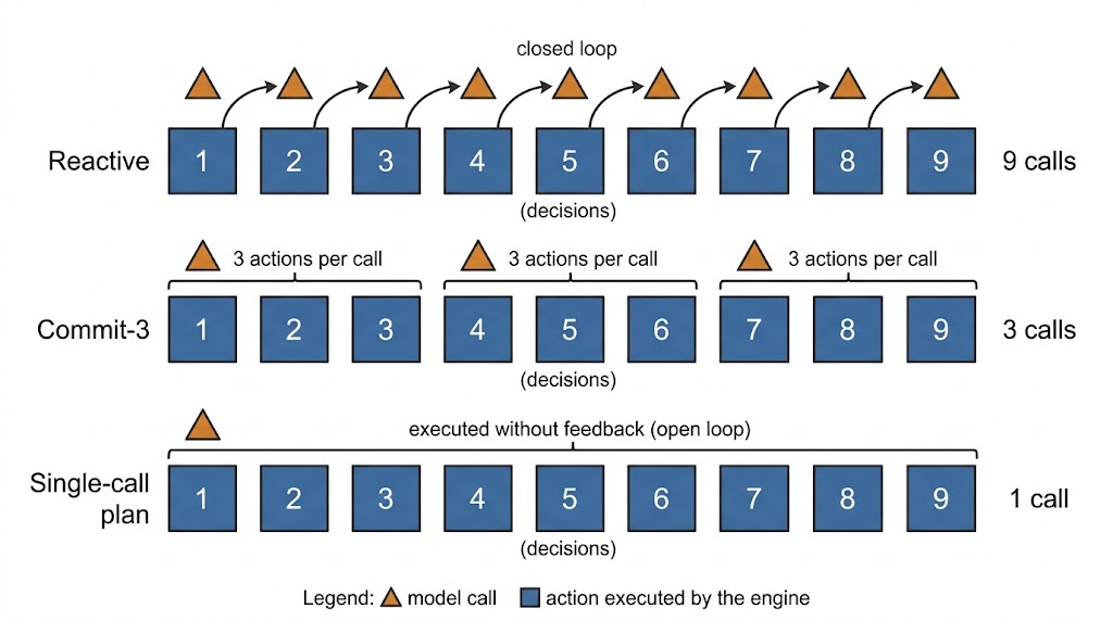
Figure 2.2: Planning horizons over nine decisions. A reactive agent calls the model at every decision (closed loop); a commit- agent calls it every decisions; an agent with a single-call plan calls it once and executes the rest without feedback (open loop).
Long episodes make this trade-off sharper. The consequence of a decision may appear many steps later, for example when a key spent early is missing at a door near the end. Errors also compound: an agent that succeeds at each step with probability 0.99 completes a 100-step episode without error with probability .
In the following section, the question changes from how an agent acts to how its behaviour can be improved.
Further reading: Russell and Norvig (2021, Ch. 2) define agents and environments; Sumers et al. (2024) give a framework for language agents.
2.5 From Weight Optimisation to Prompt Optimisation
A model's behaviour can be changed in two places: in its parameters or in its input. Fine-tuning changes the parameters by continuing training on task-specific data, typically pairs of inputs and desired outputs. It requires access to the parameters and substantial computing hardware.
Reinforcement learning (RL) is used when desired outputs are not available but outcomes can be scored. The agent acts, receives a scalar reward, and its policy is changed so that high-reward actions become more likely (Sutton and Barto, 2018). For LLMs, the policy is the model itself, and the change is a gradient step on its parameters. Reinforcement learning from human feedback (RLHF) trains a reward model on human preference judgements and then optimises the LLM against it with Proximal Policy Optimization (Christiano et al., 2017; Schulman et al., 2017; Ouyang et al., 2022).
Group Relative Policy Optimization (GRPO; Shao et al., 2024) simplifies this procedure. For each input it samples a group of outputs, scores each with a reward , and uses each output's standing within its group as the learning signal:
Outputs better than their group are made more likely, worse ones less likely, without a separate network that estimates expected rewards. GRPO was used to train DeepSeek-R1 (Guo et al., 2025). Like other policy-gradient methods, it learns only from the scalar score: the optimiser does not see why an output failed.
When a model is accessed through a service, as in the main experiments of this thesis, its parameters cannot be changed. The only remaining parameter is the prompt , and the policy becomes with fixed weights. The outer loop stays the same: run episodes, observe outcomes, update the parameter, repeat. The update itself differs. A prompt is text, and text can be revised by a model that has read what went wrong. Ramnath et al. (2025) accordingly classify prompt optimisers first by the feedback they use: a scalar score, or a textual description of the failure.
In the following section, the methods that optimise prompts automatically are introduced.
Further reading: Sutton and Barto (2018) is the standard textbook on reinforcement learning; Shao et al. (2024) introduce GRPO.
2.6 Automatic Prompt Optimisation and GEPA
Automatic prompt optimisation (APO) replaces the manual rewriting of prompts with a search over prompt text (Ramnath et al., 2025). Methods that use a scalar score generate many candidate prompts and keep those that score well. APE samples candidate instructions from an LLM and filters them by score (Zhou, Y. et al., 2023). OPRO shows an LLM the history of prompts and their scores and asks for a better one (Yang et al., 2024). Promptbreeder and EvoPrompt evolve populations of prompts with mutation and crossover (Fernando et al., 2024; Guo et al., 2024). MIPROv2 searches over instructions and examples with Bayesian optimisation (Opsahl-Ong et al., 2024). Methods that use textual feedback ask an LLM to criticise a failed output and to revise the prompt accordingly. ProTeGi calls such criticisms "textual gradients" (Pryzant et al., 2023), and TextGrad propagates them through programs of several LLM calls (Yuksekgonul et al., 2024).
2.6.1 GEPA
GEPA (Agrawal et al., 2025) is a textual-feedback optimiser that uses the full record of an episode, its trace, as feedback. It maintains a pool of candidate prompts and repeats five steps (Figure 2.3):
- Select a parent prompt from the pool.
- Roll out the parent on a small batch of task instances and record, for each, the score and the trace.
- Reflect: a second language model reads the parent prompt, the traces and the scores, diagnoses what went wrong, and writes a revised prompt. Agrawal et al. (2025) call this model the reflection model; this thesis calls it the teacher.
- Accept the revision if it scores better on the same batch, then evaluate it on a validation set and add it to the pool.
- Merge (optional): combine two candidates that succeed on different instances into one prompt.
GEPA, Promptbreeder and EvoPrompt are evolutionary algorithms in the standard sense (Eiben and Smith, 2015): a population of candidate solutions, variation operators that produce new candidates, and selection by a fitness measure. In prompt evolution the candidate is the prompt text and mutation is a rewrite by a language model. Recombination is the merge of two prompts, and fitness is the score of the prompt's episodes. GEPA's distinctive choices are that mutation is guided by traces rather than random, and that selection keeps every candidate that is best on at least one instance. The smallest evolutionary algorithm, the (1+1) scheme, keeps a single parent, produces one offspring per generation and keeps whichever of the two is fitter; in this thesis, a tie goes to the offspring.
Parent selection uses the Pareto frontier of the pool: the set of candidates that are the best on at least one validation instance. Sampling from this set keeps alternative strategies alive when different instances reward different behaviour. The frontier and the merge step therefore operate across task instances; Section 5.7 describes which parts of the algorithm are used in this thesis. Across six benchmark tasks, Agrawal et al. (2025) report that GEPA outperforms GRPO by 6 % on average and by up to 20 % while using up to 35 times fewer rollouts. GEPA also outperforms MIPROv2 by more than 10 %.
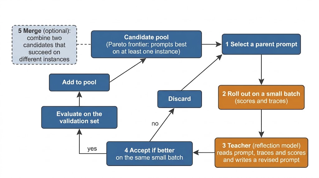
Figure 2.3: The GEPA optimisation loop as described by Agrawal et al. (2025).
The output of GEPA is a prompt that a person can read and compare with its predecessor. The same holds for every prompt produced by reflective prompt evolution: the result can be read and compared line by line.
In the following section, the chapter turns from learning-based methods to exact search, which supplies the reference against which the agents are measured on single floors.
Further reading: Ramnath et al. (2025) survey automatic prompt optimisation; Agrawal et al. (2025) describe GEPA in full.
2.7 State-Space Search and Exact Solvers
A problem in which the outcome of every action is fully determined can be described as a state space. A state is a complete description of the situation from which the future can be computed. For the game in this thesis, a state consists of the hero's position, hit points (HP), attack (ATK), defence (DEF), magic defence, gold, experience, keys, and the set of tiles already cleared. Each legal action leads from a state to exactly one successor state. Starting from the initial state and expanding all successors repeatedly yields a search tree, whose leaves are won, lost or unfinished games (Russell and Norvig, 2021).
Breadth-first search (BFS) expands the tree level by level, so that every state reachable in actions is visited before any state that needs . Exploring the whole tree guarantees that the best leaf is found, here the win with the most HP remaining; a solver with this guarantee is called exact. The difficulty is size: with choices per step and steps, the tree has on the order of leaves. Exact solvers therefore rely on pruning, the safe removal of states that cannot lead to a better result. The central pruning rule is dominance. If two states have the same position and the same cleared tiles, and one is at least as good as the other in every attribute and every key colour, the worse one can be discarded. Every continuation of it is available to the better one with at least the same outcome. Applied correctly, dominance pruning preserves exactness; Chapter 4 shows how an incorrect implementation of this rule in a published solver discards the optimum.
A rule-based heuristic, by contrast, chooses each action by a fixed rule, for example "take the cheapest available fight". It needs no search, but it offers no guarantee: a locally cheap action can make the game unwinnable later.
Figure 2.4 illustrates these concepts on the upper part of the simple floor, a test map of a published solver for the game and the running example of this thesis (Chapter 4). The hero starts at the top and first picks up the yellow key directly below. It then faces four choices: three monsters (a Slime Lord, a Red Slime and a Black Slime) and a yellow door that the key opens. The exact solver evaluates every continuation of each choice. The highest final HP still reachable from a state is its state value. Fighting the Black Slime first keeps the state value at 13 HP; each of the other three choices makes the floor unwinnable. Three of the options look cheap: the door costs no HP, and the Red Slime costs only 1 HP more than the Black Slime. Only search, or equivalent reasoning about the keys and fights ahead, separates them.
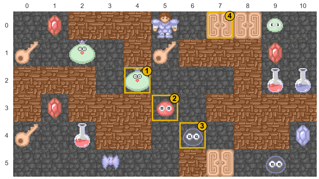
Figure 2.4: Upper part of the simple floor (rows 0 to 5 of 11), drawn with the game's own tiles. Positions are (x, y), with column x counted from the left and row y from the top, both starting at 0. The hero starts at (5,0) and first picks up the yellow key at (5,1). The four choices are then marked: (1) the Slime Lord (4,2), (2) the Red Slime (5,3), (3) the Black Slime (6,4) and (4) the yellow door (7,0). The state value after each choice, the highest final HP the exact solver can still reach, is 13 HP after choice 3 and none after the other three (the boss can no longer be defeated). Other objects: yellow keys and doors, red gems (+1 ATK), blue gems (+1 DEF), red and blue potions (+75 and +200 HP), a Green Slime (9,0), a second Slime Lord (2,1), a Bat (3,5) and a second Black Slime (9,5); brown tiles are walls. try this decision
In the following chapter, the work that applies these concepts to games, to planning with LLMs and to prompt optimisation is reviewed, and the gap addressed by this thesis is identified.
Further reading: Russell and Norvig (2021, Ch. 3) introduce state spaces and uninformed search.